Excel: Managing Data - Macros, Lists, and Validation

Creating Cell Drop Down Menus and Adding a Condition

From time to time you may need to have a list of options for your clients to choose from; this is

especially true when creating contracts, invoices, and forms in Excel. For example, you can have a cell

activate as a drop down with the options of 1 month, 3 months, 6 months, or 12 months when creating

a lease contract. Then you can have the “amount due each

month” cell auto-populate with the correct rent amount

without having to type the information in yourself.

 Click into cell A41 in the table spreadsheet.

 Type “1 month” in A41, “3 months” in A42, “6

months” in A43, and “12 months” in A44.

 Click in cell B41. (We are going to place the list

here.)

 Go the Data Tab and click Data Validation.

 Click Data Validation again.

 The Data Validation meu will appear.

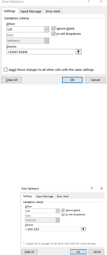
 In the Allow -> List.

 Then either type the absolute formula =$A$41:$A$44

or select the cells after clicking in cell A41- A44.

 Make sure In-cell dropdown is selected. This will allow us to apply this drop down anywhere on

the spreadsheet.

 Click Ok.

 Now when you click into cell B44, you will see the droplist. You can choose any of the options.

 Let’s apply a conditional formula (review the breadcrumb conditional formula from a previous

workshop).

 In cell C43 type: =IF(B41=”1 month”,”$400 per month”,IF(B41=”3 months”,”$600 per

month”,IF(B41=”6 months”,”$900 per month”,IF(B41=”12 months”,”1200 per month”,”Write

In”))))

 Now cell C43 will update as the information changes in cell C43! What we are saying with this

formula is what lease by month a person signs, the appropriate rent will apply in the cell C43.

Multi-Layered Lists

You can create multi-layered lists with a drop down to auto-input information into a table or data set.

 Go to the Cell List spreadsheet.

 Let’s create list by region and another list of states by region.

 Click the letter A to highlight all of column A.

 Go to the Data tab -> Data Validation -> Data Validation.

 Change Allow to List and Source: Highlight the cells that has

the region information (E1 – J1)

 Click Ok.

 Now click into Cell A2 and you can see the drop down list.

**This list will apply to the entire column since we

highlighted the column when creating the list**

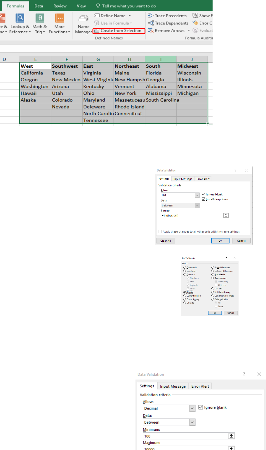
 To add the corresponding states to the region in column B, highlight all columns and rows that

contain the data you need – include blank cells in columns if some columns don’t have as long a

list. For this example, highlight cells E1 – J9. This should highlight all cells that has data.

 Go to the Formulas tab -> Create from Selection



 In the Create Names from Selection box, put a check mark Only in Top Row.

 As a sidenote, look at your NameBox on the top left corner when you click in any cell that is

highlighted. It should change to the corresponding Region. Hopefully, this is a reminder from the

first Basic Excel workshop.

 Click on B to highlight all of column B.

 Go to the Formulas tab -> Data Validation -> Data

Validation.

 Change Allow to List.

 In the Source type the formula: =indirect(A1) *This is

telling Excel to go back to the list in cell A1 to correspond

to the data in column B.

 Click OK.

 You more than likely will get an error “The Source

currently evaluates to an error. Do you want to

continue?” Click Yes.

 Click in cell A2, and choose West.

 Click in cell B2, and the list should only show states in the West.

 Now, to remove the blank spaces in the list of States, highlight all

the state data, without the header information. No: West,

Southwest, East, etc. (Only cells E2 – J9)

 Go to the Home tab -> Find and Select -> Go to Special

 In the Go To Special select Blanks.

 Click OK.

 Right click in any of the highlighted blank cells -> Delete.

 Select Shift cells up.

 Now test the state drop downs to see if you get any blank spaces at the end of the lists. They

should now be removed.

Working with Data with Controls

Data Validation allows you to control the data that goes

into each cell. It also allows you to force your data entry

clients to format date the way you want.

 Go to the Macro spreadsheet.

 Click on the letter F to highlight the entire

column

 Go to the Data tab -> Data Validation -> Data

Validation

 Change Allow to Decimal.

 Change minimum to 100 and maximum to 10000.

 Click on the Input Message tab.

 This is where we can add a “comment-like”

message when we hover over any cell in column

F – in Title: Range Input Message: Only numbers

between 1 and 10000.

 Click on the Error Alert tab. This is where you can customize the error messages your data entry

people will see if they type something wrong. In title: Try Again –

Error Message: Only numbers between 1 and 10000.

 Click Ok.

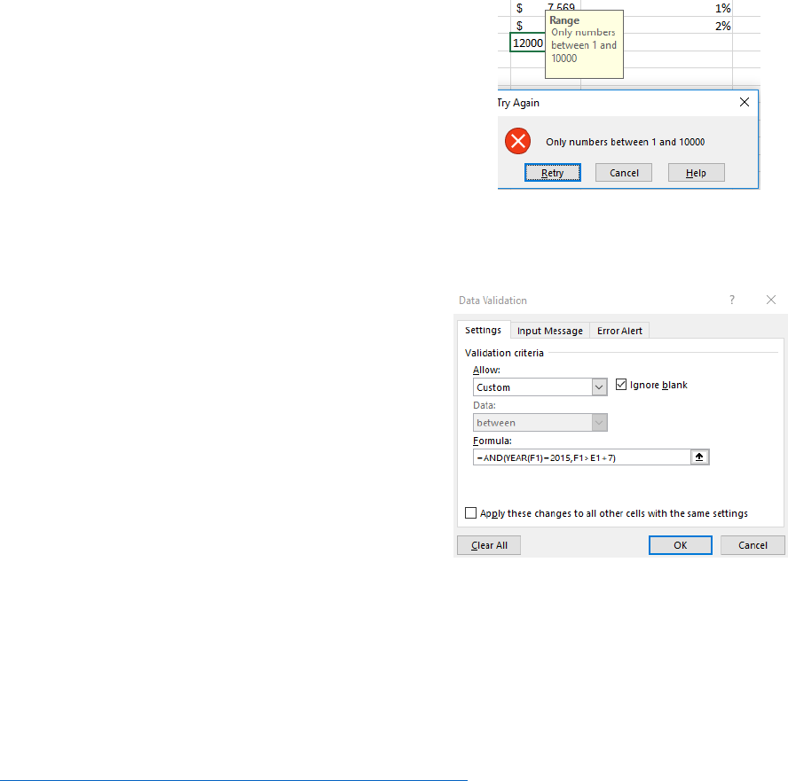
 Go to cell F30 and type 12000. You should get the error message

we just assigned.

 In the same cell, type 5000. It should work now.

 ***Look at all the data options you have in the Data Validation ->

Allow options. You can customize and format numbers, decimals,

dates, time, etc.

Data Controls with Formulas

 Go to the Date spreadsheet.

 Let’s assume we are going to put dates into column F that is

at least 7 days from the days in column E. You typically will

see this when your business provides shipping and handling.

 Click on the letter F to highlight all of column F.

 Go to the Data tab -> Data Validation -> Data Validation.

 In the Allow -> Custom.

 In the Formula box, type: =AND(YEAR(F1)=2015,F1>E1+7)

***In a previous workshop, we discussed AND/OR and date

formulas. We are just combining two.

 Click Ok. ***You may get the error “A named range you

specified cannot be found” – Click OK.

 Now type 1/16/2015 in cell F2. You should get an error

because it is not at least seven days after 1/15/2015.

 Now type 1/25/2015. It should work!

Forecast Spreadsheets

Typically investors and accountants will use the forecast feature when looking at stock or other

investment information. In this case, let’s forecast Google Stock by month.

 Go to: https://finance.yahoo.com/quote/GOOG/history?p=GOOG

 Change Frequency to Monthly

 Click Apply

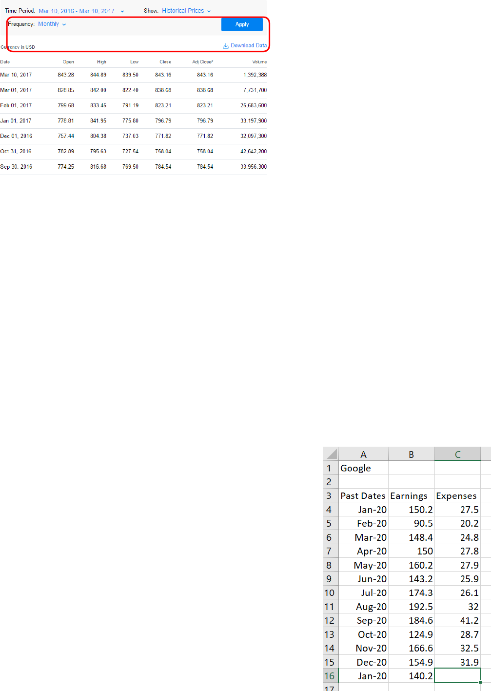
 Now click Download Data. This will export the data into Excel.

 Highlight columns A and E - the Date and Close information.

 Go to the Data tab -> Forecast Sheet

 You should get a preview pop-up window with a chart forecasting Google Stock.

 At the bottom of the Create Forecast Worksheet change Forecast End to 1/1/2018.

 Click Options

 In the Options menu, you can set data to manipulate the data in the forecast:

Confidence Interval: is important to predict forecast accuracy. Typically, the closer to 0% the

more confidence you have in the prediction. That is why it is at 95%; Excel is giving you more of

a spread. Try lowering the Confidence Interval and notice the spread shrink.

Seasonality: is the number or periods in which you are looking for data. In our example, we are

looking at Google stock by months so the seasonality is 12. You can change that here if you are

looking for a different period.

Include Forecast Statistics: this will add more statistical information when you create a

worksheet on the data by adding a table using the statistics function FORECAST.ETS.STAT that

will include measures and errors when analyzing the data. In other words, forecast by

smoothing.

Fill Missing Points Using: Excel will average out any missing points that is missing from the data.

That is why Interpolation is selected. If you do not want that information forecasted, select Zero

in our example, leave it Interpolation.

Aggregate Duplicates Using: Excel will default average out data in the same time-period. You

can change that here to a different algorithm here.

 Click Create.

 Now the forecasted data will appear in a new sheet. Typically, you are

going to look at the future numbers at the end of the inserted table.

Forecast Statistical Formulas

 Forecast formulas are typically used as part of Excel’s financial modeling

set of functions that calculate the statistical value of a forecast. In other

words, based on past earnings and expenses, you can forecast the future

amounts.

 For this example, follow the instructor’s lesson in exporting a company’s

balance sheet from Mergent Online in Excel. (This is a library database)

 Click in cell C16

 The formula we will use is =FORECAST(B16,B4:B15,C4:C15)

 What this formula calculate is the forcasting the expenses for the month

of January 2020.

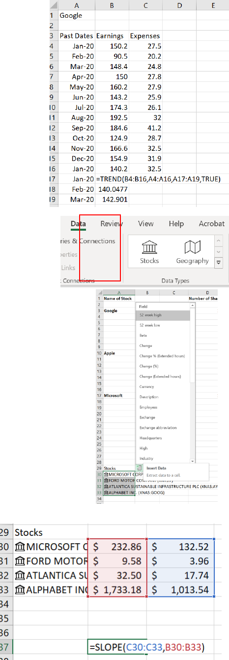
Trends

Going back to the formulas class, the trend formula will calculate the

linear trend line to known arrays. (Arrays exercises in the formulas

class) What this formula attempts is to calculate future trends or

predict future data such as revenue or earnings of a company. For

this exercise, let’s predict the earnings from Jan 20 – Mar 20.

 Add in Jan, Feb, and Mar 2020 in the spreadsheet.

 In cell B17, type =TREND(B4:B16,A4:A16,A17:A19,TRUE)

Stocks!

 Finding and auto-updating stock information in Excel 365 is really

easy.

 Go to the Stocks spreadsheet

 Highlight cells A30 – A33.

 In the Data Tab, click the Stocks button.

 This will automatically link the stocks to Excel and will auto update

when the market is open.

 At the top right of the highlight, there is a button called “Insert Data”

 Choose 52 week High, 52 week Low, Beta, Change, Currency, Ticker

Symbol, Industry, P/E

 *Note: if you are using an older version of Excel, you will need to bring in

stock information through the File -> Options -> Data Tab -> Stocks

Portfolio Slope

The Slope formula is used to calculate the beta of a particular

stock or even a portfolio of stocks. Let’s find the beta of the

stocks above.

 We will use the 52-week high and low information.

 In cell C37, type: =SLOPE(C30:C33,B30:B33)

 This should give you the beta of the stocks found.

Macros

Macros in Excel are in short, a recording of keystrokes. Beyond simple recording, you can use macros to

automate tasks that you will use over and over. In this exercise, we will find all cells that contain

formulas with the understanding that we may use this feature in different spreadsheets or over and

over.

*From the previous workshop, bring out the Developer Tab from the

File-> Options -> Ribbon -> Developer

 Open the Stocks Spreadsheet

 Click on Cell B1

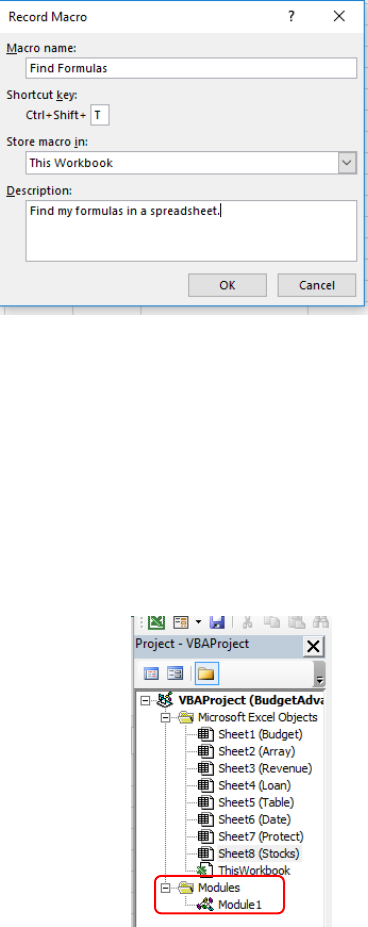
 In the Developer Tab, click on the Record Macro button.

 Change the Macro Name to “FindFormulas” – no spaces

 Change the Shortcut Key to Cntl + Shift + T (press Shift +T) to

add it as a shortcut.

 For now, keep This Workbook

 Put in a description on what the Macro will do in the

“Description” box.

 Press OK

 Go the Home Tab and click on the Find & Select button.

 Add a color to the cells by clicking on the Paint Bucket button in the Home Tab. Add a color.

 Go back to the Developer Tab and click Stop Recording.

 Click anywhere on a blank cell, and all your cells that contain formulas will be highlighted in a

color.

 Undo the cell coloring by pressing Cntl + A and select No Fill from the paint bucket button from

the Home Tab.

 Now on the spreadsheet, press Cntl + Shift + T – this will run your macro!

 Now try the Macro on a Loan spreadsheet. It should highlight your cells with formulas.

Microsoft Visual Basic for Applications Environment

Again, you do not need to know a lot about VBA code, but it is a good idea to at least

get familiar with the VBA environment.

 To quickly get to the VBA environment, you just need to press Alt + F11 or you

can Click on the Macro button in the Developer Tab.

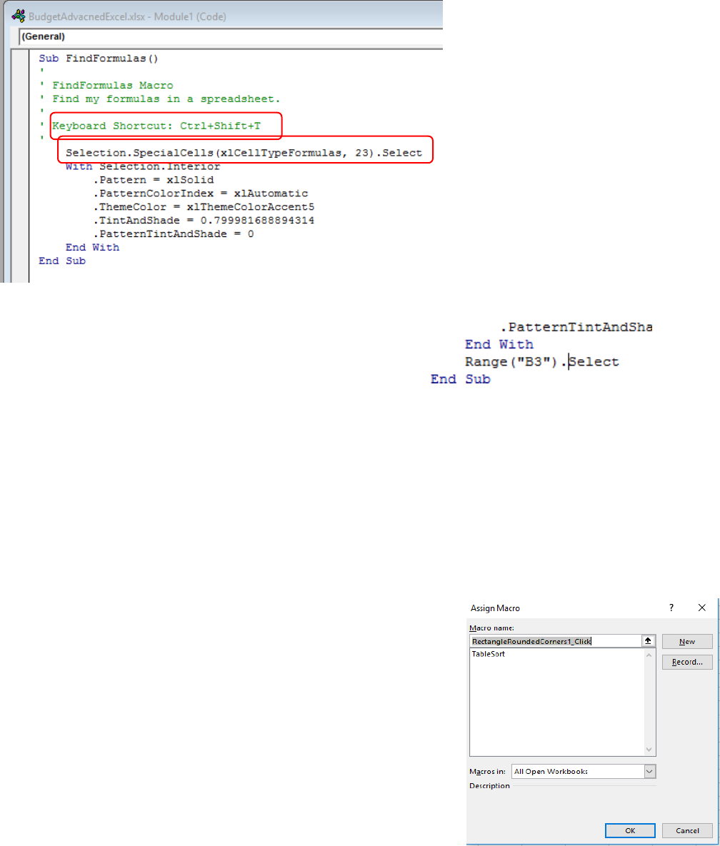
 On the left side of the screen, you will see the Project – VBAProject menu that

will contain your spreadsheets and macros.

 All your macros are saved in the folder titled: Modules

 Since we have one macro, you will see Module 1 when you click on the

Modules folder.

 Double click on Module 1 and the VBA code for the macro we created above

will appear.

 The code on the right is code to run the macro to find formulas on a spreadsheet and change

the cells to a color. *Any text in green in the code are just comments and they will not affect

anything.

 The instructor will discuss with the code means, but you can always add code to VBA scripts to

make the macro more customized.

 In this example: type Range (“B3”). Select between “End With”

and “End Sub”

 What this is going to do is move your cursor to cell B3 after the

macro is run.

 Press ALT+F11 and run the macro on the Stocks spreadsheet.

 Your cursor will end up in cell B3

Macros as Buttons

There are two ways to create buttons in Excel that will run a macro in the background that will make

tasks that much easier to process. In most cases, you will set up buttons when you must send the

spreadsheet over to data entry clients so they do not mess up data on your spreadsheet. One method is

to create a button from a shape or insert a picture or you can assign a button already made in the

Developer Tab.

 Go back to the Table spreadsheet.

 Go to the Developer Tab and click on Record Macro.

 Macro Name: SortTable

 Shortcut Key: Ctrl + Shift + Y

 Click OK.

 Highlight cells A4-A36, and in the Home Tab, click Sort A-Z

 Go back to the Developer Tab and click: Stop Recording.

 Now press the undo button on the top left of the screen to unsort the

data.

 Go to the Insert Tab -> Shapes -> Insert a rectangle

 In the rectangle, type Sort by Name

 Right-click in the rectangle and select Assign Macro

 So far, we only have one macro assigned to this worksheet, so click on TableSort and change

Marcos In to This Workbook. (Since this macro is designed for this spreadsheet, that is why we

are choosing this option)

 Click Ok.

 Click outside the button to deselect the object.

 Now when you move your mouse over the button, it should change to a finger ready to press.

Press the button, and it should sort your data. (*You can easily insert a picture and turn that

into a button what a macro. Most businesses will do this with a logo.)

 Excel already has pre-designed buttons that do tasks to help build surveys.

 In this example, let’s create a macro to print a spreadsheet and

then create a button to press to quickly print.

 Go to the Developer Tab -> Record Macro. (Name the macro

PrintArea with Cntl+Shift+G)

 Print the spreadsheet like you normally do: File -> Print -> Print.

 Go back to the Developer Tab -> Stop Recording.

 Click on the Insert Button in the Developer Tab and Select the

Button command.

 You can draw a button on the spreadsheet just like drawing a

shape.

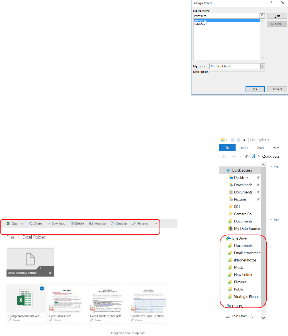
 When you draw a button, the Assign Macro menu will appear.

 Now we should have two macros.

 Click on the PrintArea and click Ok.

 Now press the button, and it should print the spreadsheet.

 You can rename the button to “Print” to add what the button will do.

OneDrive

Microsoft provides free online storage and document creation directly on the

browser with an account. (Outlook, Hotmail, Xbox, MSN, etc.) If you have a

Microsoft account – including your student Outlook account – you already have a

OneDrive account. Login by going to www.onedrive.com and use your Microsoft

PC, Onedrive is already on your File Explorer.)

With OneDrive, you can also share single documents or entire folders with specific

people or with the public.