
Modeling of Football Match Outcomes with Expected
Goals Statistic
Adan Partida
1
, Anastasia Martinez
1
, Cody Durrer
1
, Oscar Gutierrez
1
and Filippo Posta
1
1
Estrella Mountain Community College, Avondale, AZ, USA
DOI: https://doi.org/10.47611/jsr.v10i1.1116
ABSTRACT
Aim. Our research examined the predictive capabilities of mathematical models that are solely based on the expected
goal statistics obtained from a publicly available database.
Method. We collected match and expected goals data for 310 matches from three European Leagues (Bundesliga, La
Liga, and Serie A). We created three probabilistic models based on the expected goals statistic and compared them
with two well-established probabilistic models using binomial deviance, squared error, and profitability in the betting
market as evaluation metrics.
Results. Our best model adjusted the expected goal statistics for homefield advantage and outperformed the two prob-
abilistic models used for comparison. Two of our models were profitable under certain betting conditions.
Limitations. Our models explored a simplistic integration of expected goals into a Poisson based probabilistic model
and did not include other contributing factors such as a team’s defensive prowess. The number of games simulated
was also limited due to the premature closure of the European Leagues due to the COVID-19 pandemic.
Conclusions. The use of a probabilistic model based solely on expected goals score statistic can provide some mean-
ingful insight into forecasting the outcome of a football match and can develop useful betting strategies.
Introduction
Modern engineering and computer science allow for the accumulation of relevant measurements across many fields
of interest. These measurements are combined into datasets that are mined to identify patterns used to answer field
specific questions. Data analytics has become fundamental in all aspects of the sports industry (Mondello & Kamke
2014). Sport organizations use predictive analytics to improve their odds on the court, injury prevention, ticket pricing,
and payroll optimization (Link, 2018; Dobson et al., 2001). Even governing bodies, such as the Federation Internatio-
nale de Football Association (FIFA), use data analytics to determine rankings in seeding decisions that can have major
financial implications (Monks & Husch, 2009). The betting industry is another industry that has been at the forefront
of the data analytics revolution. Oddsmakers use data to improve the calculations of odds but also to provide new
betting opportunities for their customers such as live betting (Pearson, 2017). The sheer economical size of the sports
and betting industries has created a fertile and extremely competitive ground for scientists to create new ways to
measure hard to quantify features (e.g., effort, clutch) and to develop predictive models that can lead to economical
and on-court advantages (Cintia et al., 2015; Link, 2018). These new data and predictive models use approaches from
many fields of science, from engineering to finance and medicine, and often lead to extremely advanced and complex
algorithms.
As the most global sport, football (soccer in the US) is an excellent case study for the analysis and develop-
ment of sports analytics. The game has been studied in depth for many years by fans and scholars alike and there are
many publicly available databases that can be used as resources for game data (Rein & Memmert, 2016; Cintia et al.,
Volume 10 Issue 1 (2021)
ISSN: 2167-1907
www.JSR.org
1

2015; Link, 2018). The football betting industry is also a well-established worldwide phenomenon grossing billions
of dollars.
Interest in predicting football match outcomes is matching the popularity of the sport and can be summarized
into two overlapping trends: creating new statistics and developing computational algorithms that take advantage of
the throve of available data. One of the most promising statistics is expected goals (xG). xG was first introduced for
professional ice hockey (Macdonald, 2012) and has since become ubiquitous in football (Eggels et al., 2016). xG data
are often used as one of the features of interest to create computational models involving advanced data science tech-
niques such as artificial neural networks (Hucaljuk & Rakipovic, 2011) or in combination with other factors (e.g.,
payroll, match attendance, etc.) to create sophisticated rating systems (www.fivethirtyeight.com).
Our study explored the possibility of using publicly available data to create straightforward mathematical
models to predict the most likely outcome of a football match. Our analytical modeling approach can be applied to
any football match. For practicality, we collected data from 3 European leagues (German “Bundesliga”, Italian “Serie
A”, and “Spanish Liga”). The models are straightforward because they are based off the well-known football principle
that it is harder to score than to defend. Therefore, our models focus on predicting goals by team. In our approach,
goals scored by a team are predicted almost independently from a team’s opposition. We only used game related data
instead of trying to incorporate too many variables such as form, injuries, line-up, game importance, etc.
To assess the quality of our models, we used the probabilities used by Las Vegas oddsmakers as well as a
well-established model from the 538 website (www.fivethirtyeight.com) as “gold standards” for comparison. In addi-
tion to studying our models’ predictive capabilities, we also analyzed if the models could be profitable under some
simple betting rules and compared this profitability with the gold standards.
The idea behind this approach to predicting football math outcomes is not new. Our first model in this study
is a straightforward starting point in the implementation of any xG based predictive model. The novelty of our study
is based on the investigation of simple changes to the basic model and how they compare to more advanced models,
as well as the use of publicly available data that which allow for ease of replication and further exploration.
Materials and Methods
We collected publicly available data to create simple but highly interpretable statistical models and we also used
publicly available data to compare the predictive abilities of our models. The workflow of our study is summarized in
Figure 1 and describe in more details below.
Volume 10 Issue 1 (2021)
ISSN: 2167-1907
www.JSR.org
2
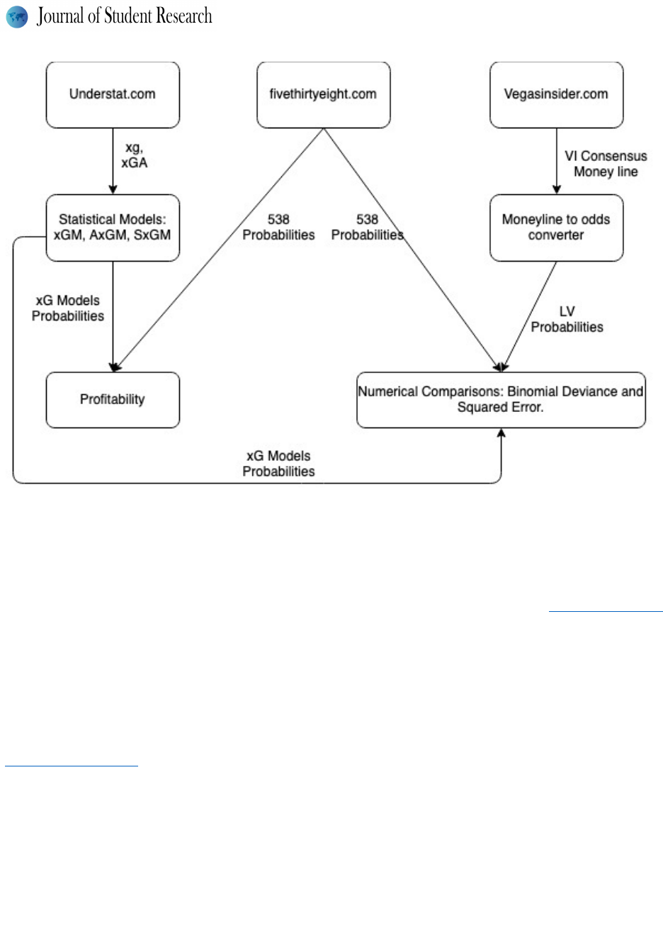
Fi gure 1 – Workflow of the study from data collection to qualitative comparison and profitability.
Dataset
We built a Microsoft Excel spreadsheet of football data during the 2019/20 football seasons for three European
leagues: Bundesliga (Germany), La Liga (Spain), and Serie A (Italy). We wanted to use publicly available data in-
cluding the xG statistic derived solely from physical football events. We selected the website www.understat.com
(Understat) for their “detailed XG statistics trained using neural networks on more than 100,000 shots”. Understat
uses on-field statistics of players such as shots, passes, goals, appearances and minutes played to build the xG statistic.
From Understat, we collected weekly team fixtures including team names, xG scored (xG) and allowed (xGA) for
each team in the league. We also collected the number of matches (M) played by each team at the time of collection.
We collected this data on a weekly basis beginning on Week 7 of each league and continuing until the league suspen-
sion due to the COVID-19 pandemic. For comparison purposes, we collected the predictive match probabilities created
by 538 for the same fixtures in our dataset. Finally, we collected match odds from the Vegas Insider website
(www.vegasinsider.com). Within the website, we picked the odds in the “VI Consensus” column. These odds consist
of the betting line that occurs most frequently among Las Vegas and Global bookmakers followed by Vegas Insider.
We used Understat’s data to build our predictive models and the data from 538 and LV to compare the predictive
capabilities of our models. The final spreadsheet contained 310 matches from the 3 European Leagues.
Predictive Models
xG Model (xGM) - Our starting model used two assumptions: that the best predictor of the numbers of goals is the xG
statistic, and that the number of goals scored by a team follows a Poisson distribution. xG represents the number of
goals a football team is expected to score in a match against an opponent based on the quantity and quality of chances
created (Eggels et al., 2016).
Volume 10 Issue 1 (2021)
ISSN: 2167-1907
www.JSR.org
3
We used the xG statistic as input for the Poisson distribution to generate goal scoring probabilities that were
combined into probabilities of a home, away, or draw outcome. The Poisson distribution provides a valid approxima-
tion capable of representing the number of goals scored in a football match (Karlis & Ntzoufras, 2003).
The xGM model calculates the probability of a team scoring a certain number of goals by using the following Poisson
formula:
() =
!
where P(k) is the Poisson probability that exactly k goals are scored in a match.
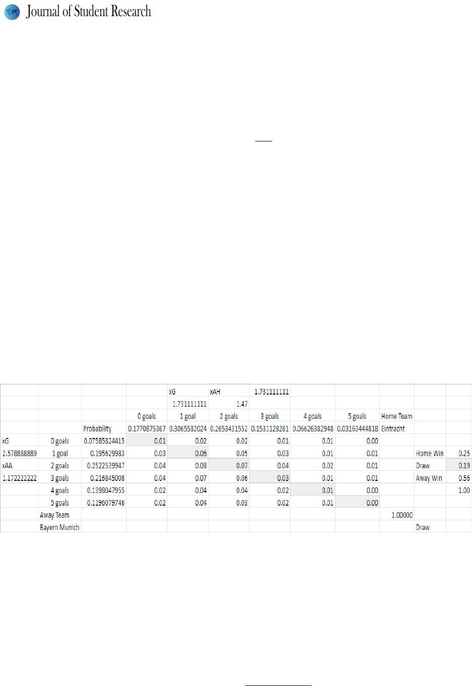
The process of building the probability of having a home win, away win or draw from this model is depicted in Figure
1. The figure uses as example a match in the Bundesliga between Eintracht Frankfurt (home team) and Bayern Munich
(away team). For each team, we calculated P(k) with k going from 0 to 5+ (the 5 goals or more case being 1 minus
the sum of all of the previous probabilities) with the above formula. The home team probabilities are aligned horizon-
tally, and the away team probabilities are aligned vertically. Each cell on the table below and to the right of the goal
probabilities shows the probability of an exact score obtained by multiplying the appropriate probabilities. For exam-
ple, the probability of a 1-1 draw is obtained by multiplying the probability of the home team scoring 1 goal
(P(1)=0.02) and the probability of the away team scoring also 1 goal (P(1)=0.03). Therefore, the probability of Ein-
tracht and Bayern tying 1-1 is 0.06. We calculated the probability of a draw by summing all of the probabilities where
the home team and away team score the same number of goals (shaded diagonal in Figure 2). For the home and away
team winning probabilities, we sum all of the probabilities for the respective outcome. We calculated the draw prob-
ability as the difference between 1 and the sum of the home and away win probabilities to account for rounding errors
and to verify that the sum of the probabilities of the three outcomes is 1.
Fi gure 2 - Sample probability matrix for the xGM. The shaded cells show the probabilities of 0-0, 1-1, 2-2, 3-3, 4-4,
or 5+ - 5+ draws, respectively. Their sum represents the probability that the match ends in a draw according to the
xGM.
Scaled xG model (SxGM) - The xG model does not take into consideration the opposition. We hypothesized that a
better model would include the effect of the opposing team defense. We created a scaled version of the xG model
(SxGM). In this model, the input parameter for the Poisson probability distribution consists of a scaled version of xG.
In particular, xG statistics are scaled by the expected goals allowed (xGA) by the opposing team. For the SxGM the
probability that a team scores k goals is given by:
() =
(
)
!
Volume 10 Issue 1 (2021)
ISSN: 2167-1907
www.JSR.org
4

Where
is the expected goals per game allowed by the opposing team. The match outcome probabilities are
calculated analogously to the xGM
Adjusted xG model (AxGM) - In this model, the input parameter for the Poisson probability distribution consists of an
adjusted version of xG. Expected goals statistics are adjusted by adding a coefficient (
) that represents league-
based home-field advantage.
is calculated by taking the mean difference of xG overall versus xG at-home over
the past 5 years. For this adjusted model the probability that a team scores k goals is given by:
() =
(
)
(+
)
!
To validate our choice of
we ran a mean comparison analysis of the goal distributions, we calculated 95% confi-
dence intervals of the difference of the means, and we computed the effect sizes using Cohen’s D (Cumming, 2014).
All of this was done separately for each league.
Gold Standards
To test the performance of our three models we compared them to the predictions of popular statistics website 538
and the Las Vegas spreads published by Vegas Insider. 538 is an established statistical analysis website with data on
over 550,000 football matches going as far back as 1888 derived from ESPN’s database and the Engofootballdata
GitHub repository (Jayboice, 2018). This large sample size of football match data allows 538’s predictive analytics
method to benefit from multiple adjustments to corresponding probabilities in their data matrix as new games are
played. 538’s model accounts for off-field parameters such as injuries, salaries, and match importance. Vegas Insider
is a collection of spreads generated from multiple sportsbooks. We chose the VI Consensus sportsbook as the gold
standard for betting as it is an aggregate of the most common betting line that appears among the Las Vegas and
Global sportsbooks and therefore represents the average betting odds. Sports books such as the ones used in Las Vegas
create power ratings to compute and order teams against each other using a variety of variables that go beyond on-
field statistics (Kramer, 2017). Power ratings is the industry term for analytics based on game factors and are no
different than the metrics derived from 538. Of course, no two statistical methods are exactly alike but keeping as
many computational steps as similar as possible allows for a fairer comparison and is why our group considers 538
and Vegas Insider to be gold standards for comparison.
Note that the Vegas odds are not probabilities, but money-lines. To transform them into probabilities we used the
following formula:
(
)
=
100
(
100 +
)
> 0
(
10
0
)
< 0
Where money line represents the odds for either a home win, draw, or away win, and the is the amount that the
bookmakers charge each bettor for the “right” to place the bet. For our dataset it ranges between 1.03 and 1.07.
Through the above formula we were able to obtain a decimal value matching the format of our models and 538’s.
Model performance metrics
We wanted to test the predictive ability of our models as well as their ability to be profitable in the betting market.
Therefore, we conducted three separate accuracy studies to compare the performance of our models among themselves
and with the gold standards. One of the measures we used is the binomial deviance error across all games in each
league. Binomial deviance error is given by
Volume 10 Issue 1 (2021)
ISSN: 2167-1907
www.JSR.org
5

(
+ (1
)
(1
))
where
is either 0 (home win), 0.5 (draw), or 1 (away win) and p represents the probability of the outcome (Lasek et
al., 2013). For the example in Figure 2, the binomial deviance error if the game ended in a draw would have been
0.5
(
0.19
)
+
(
1 0.5
)
(
1 0.19
)
0.406.
We also calculated the squared error of the prediction by using the formula:
(
)
where the variables have the same meaning as the binomial deviance formula (Lasek et al., 2013).
Finally, we explored the profitability of our three models and 538 by incorporating three betting strategies and calcu-
lating their financial outcomes. The three strategies consisted of betting on all games by choosing the match outcome
with the highest probability of success (we labeled this rule “Best” in the results section), only betting on games with
a match outcome that had a probability greater than 50% (i.e., “>50”) and only betting on games with an outcome that
has a probability greater than 70% (i.e., “>70”).
Results & Discussion
We investigated the predictive abilities of our models versus the gold standards as well as their profitability. Gold-
standard comparisons using binomial deviance error and the squared error of prediction from the 310 matches in the
dataset are shown in Figures (3) and (4).
The AxGM model is the model with the best accuracy with respect to binomial deviance error among our
models. Its mean error is 0.298 ± 0.118 versus the xGM mean binomial deviance error of 0.356 ± 0.132 and the SxGM
mean binomial deviance error of 0.370 ± 0.204. These results suggest that adjusting expected goals statistics for
home/away splits improves model predictive capabilities more than adjusting for the opposition’s defensive capabili-
ties. The error reduction due to adjusting for home field is about 16%. In addition, taking into account the opposition’s
defensive abilities does not reduce the deviance error (there is actually a 1.5% increase on average). AxGM is also the
best performing model when compared to the gold standards and also the one with the least variation. The 538 mean
binomial deviance error of 0.302 ± 0.145 is about 1.2% worse on average than our best model. The Las Vegas mean
binomial deviance error of 0.328 ± 0.189 is 9.1% worse than AxGM with a significantly higher standard deviation.
The other two of the xG models perform worse than the gold standards.
We also looked at the accuracy in predicting individual leagues. The AxGM model performed the best for
Bundesliga and Serie A, while the 538 predictions are the most accurate for the Spanish Liga. These results are shown
in Table 1 and confirm the aggregate results with the interesting exception of the Italian Serie A where SxGM performs
better than xGM. This result is interesting because Italian football has always been known for its defensive prowess
and SxGM tries to account for the opposition’s defensive abilities.
Volume 10 Issue 1 (2021)
ISSN: 2167-1907
www.JSR.org
6
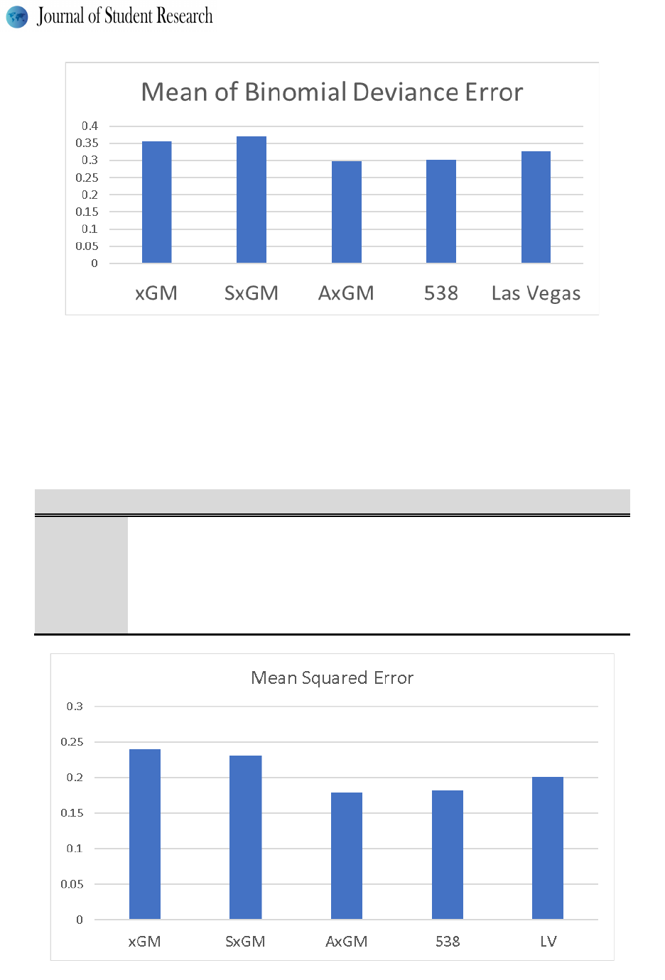
Fi gure 3 – Mean binomial deviance error results for our three models and the two gold standards.
We found similar error patterns for the squared error analysis. Figure 4 shows the mean squared error across
the 310 games and its only difference from Figure 3 consists of the squared error for the SxGM model being lower
than xGM. We also analyzed the squared error across the leagues and the results were qualitatively the same as what
we found in Table 1 for the binomial deviance (data not shown).
Table 1 – Mean and standard deviations of the binomial deviance error for statistical models organized by League.
The bolded values represent the least error for each league.
Bundesliga
Liga
Serie A
xGM
0.334 ± 0.141 0.380 ± 0.130 0.340 ± 0.123
SxGM
0.381 ± 0.219 0.401 ± 0.204 0.325 ± 0.187
AxGM
0.283 ± 0.134 0.311 ± 0.112 0.295 ± 0.113
538
0.297 ± 0.166 0.303 ± 0.144 0.307 ± 0.135
LV
0.342 ± 0.199 0.339 ± 0.215 0.311 ± 0.147
Fi gure 4 – Mean squared error results for our three models and the two gold standards.
Volume 10 Issue 1 (2021)
ISSN: 2167-1907
www.JSR.org
7

The third comparison we conducted between our predictive models and 538 were analyses of profitability.
Three separate betting strategies were investigated for our models to measure and compare profitability between each
other and against the gold standard 538. Net profits/losses together with accuracy across the 310 games in our dataset
are shown in Table 2. The numbers in Table 2 assume that a $100 bet was placed on each game that satisfied the
betting strategy. Because each model and betting strategy had different probability thresholds for placing a bet on a
game or not, the N is expressed as a range for the > 50 and > 70 betting strategies. The first number represents the
lowest number of games any model following the > 50 betting strategy bet on and the second number likewise repre-
sents the highest number of games bet on.
Table 2 - Accuracy and net profits/losses of each of our models separated across three betting strategies. The bolded
values represent the best result for each column.
Best (N=310)
> 50 (N=104-213)
> 70 (N=3-70)
Accuracy
Profit/Loss
Accuracy
Profit/Loss
Accuracy
Profit/Loss
xGM
49.35%
-$2,628.14
57.69%
-$1,611.40
66.67%
$752.67
SxGM 48.39% -$4,789.11 49.77% -$5,279.70 60.00% -$746.71
AxGM
50.00%
-$3,911.93
60.74%
-$1,352.20
70.00%
$567.00
538
50.65%
-$4,658.95 60.54% -$2,798.64 65.71% -$202.34
Betting on every match using the highest predicted probability resulted in nearly identical accuracies with
SxGM being the least accurate but only with a 2.26% difference between it and the most accurate predictor 538. SxGM
is the least accurate regardless of the betting strategy when compared to either xGM or AxGM. SxGM also reported
the highest losses out of any of our models irrespective of betting strategy as well. xGM provided the highest profits
out of every model for the best and > 70 betting strategies despite it turning out a lower accuracy than AxGM. The
reason for xGM’s profitability is due to overpredicting away wins which usually are riskier and deal higher payouts.
Our models were profitable only when betting on match outcomes with a probability greater than 70%. The
superiority of the > 70 betting strategy should come as no surprise given that only placing a bet on match outcomes
that are highly likely to occur will reduce the amount of losses than placing a bet on every match regardless of how
likely an outcome is. We see the accuracies of all our models are in line with and sometimes surpassing the accuracies
found by 538. However, 538 is consistently losing money and this is probably due to its overuse of external factors
such as team ranking in its prediction calculations. As a result, 538 is less likely to predict away and underdog wins.
These results support our hypothesis that the introduction of too much complexity in a predictive algorithm can hinder
its performance.
Conclusions
This study shows that using publicly available data combined with straightforward modeling steps lead to results that
are comparable with the more complex gold-standards used in this study. We chose these gold-standards because of
their availability as well as their popularity (538) and intuitive connection to betting (LV). It would be interesting to
compare our models to more sophisticated ones involving Machine Learning algorithms such as Artificial Neural
Networks. Our dataset did not span the whole seasons of the three Football Leagues due to the COVID-19 pandemic
and some random data collection issues. It would be important to apply these models for a whole season to confirm
these results and even identify temporal trends. The football season has various events (e.g., national team breaks,
winter breaks) happening that can significantly alter team performance.
The predictive capabilities of our models were strong enough to be profitable under certain conditions. A
further analysis of profitability in football betting could involve the investigation of the accuracy necessary to be
Volume 10 Issue 1 (2021)
ISSN: 2167-1907
www.JSR.org
8

profitable when betting all of the games as well as the use of parlays (e.g., betting multiple games at once) as betting
strategy.
It would be interesting to improve the AxGM model by expanding its incorporation of home-field advantage
and adding a team’s defensive abilities in a more meaningful way than SxGM. Implementing these changes will
require the rigorous use of more advanced modeling approaches such as regression and was beyond the goals of this
study.
References
Cintia, P., Giannotti, F., Pappalardo, L., Pedreschi, D., & Malvaldi, M. (2015, October). The
harsh rule of the goals: Data-driven performance indicators for football teams. In 2015 IEEE International Confer-
ence on Data Science and Advanced Analytics (DSAA) (pp. 1-10). IEEE.
Cumming, G. (2014). The new statistics: Why and how. Psychological science, 25(1), 7-29.
Dobson, S., Goddard, J. A., & Dobson, S. (2001). The economics of football (pp. 106-130).
Cambridge: Cambridge University Press.
Eggels, H. P., van Elk, R., & Pechenizkiy, M. (2016). Expected goals in soccer: Explaining
match results using predictive analytics. In The machine learning and data mining for
sports analytics workshop (p. 16).
Hucaljuk, J., & Rakipovic, A. (2011). Predicting football scores using machine learning techniques. 2011 Proceed-
ings of the 34th International Convention MIPRO, 1623-1627.
Karlis, D., & Ntzoufras, I. (2003). Analysis of sports data by using bivariate Poisson models.
Journal of the Royal Statistical Society: Series D (The Statistician), 52(3), 381-393.
Kramer, Adam. “Inside Look at How Las Vegas Oddsmakers Come Up with College Football
Spread.” Bleacher Report, Bleacher Report, 3 Oct. 2017,
bleacherreport.com/articles/2104561-inside-look-at-how-las-vegas-oddsmakers-come-up-with-college-football-
spread.
Jayboice. (2018, August 10). How Our Club Soccer Predictions Work. Retrieved from
https://fivethirtyeight.com/methodology/how-our-club-soccer-predictions-work/
Lasek, J., Szlávik, Z., & Bhulai, S. (2013). The predictive power of ranking systems in
association football. International Journal of Applied Pattern Recognition, 1(1), 27-46.
Link, D. (2018). Data analytics in professional soccer. Springer Vieweg, Wiesbaden.
Macdonald, B. (2012, March). An expected goals model for evaluating NHL teams and players.
In Proceedings of the 2012 MIT Sloan Sports Analytics Conference,
http://www
.sloansportsconference.com.
Mondello, M., & Kamke, C. (2014). The introduction and application of sports analytics in
professional sport organizations. Journal of Applied Sport Management, 6(2).
Volume 10 Issue 1 (2021)
ISSN: 2167-1907
www.JSR.org
9

Monks, J., & Husch, J. (2009). The impact of seeding, home continent, and hosting on FIFA
World Cup results. Journal of Sports Economics, 10(4), 391-408.
Pearson, A. (2017). How real-time analytics changes the face of the sports betting industry.
Journal of Digital & Social Media Marketing, 5(1), 61-75
Rein, R., & Memmert, D. (2016). Big data and tactical analysis in elite soccer: future challenges
and opportunities for sports science. SpringerPlus, 5(1), 1-13.
Volume 10 Issue 1 (2021)
ISSN: 2167-1907
www.JSR.org
10
